This site is under development. More capability areas and case studies are being added.

Physics-informed analytics

Seven capability areas

Each area below is a direction of work grounded in established methods. Where a PhyAnalytics study exists, it is linked; otherwise the figure is a computed method demonstration, labelled as such.

01 / Model Calibration

Infer uncertain model parameters from observations.

The problemPhysical models carry parameters that cannot be measured directly: a temperature coefficient, a reaction rate, a material property. Calibration estimates them from data and states how tightly the data constrain them.
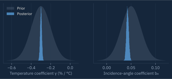
Evidence: CASE / 001

Prior and posterior distributions for a solar module's temperature coefficient and incidence-angle coefficient; both posteriors are much narrower than the priors.
From CASE / 001: the data narrow a physics-based prior for each coefficient into a tight posterior.

02 / Surrogate Modelling

Construct efficient approximations of computationally expensive models.

The problemWhen each simulation is costly, exploring parameters, calibrating or optimising becomes impractical. A statistical emulator trained on a few runs predicts new outputs quickly, together with an estimate of its own error.
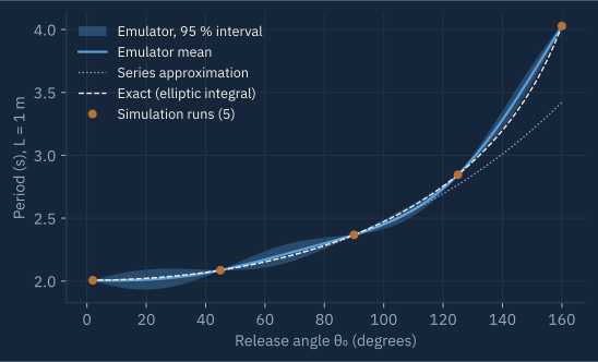
Pendulum period against release angle: five simulation runs, an emulator mean with a 95 % interval, the exact curve and a series approximation that fails at large angles.
Method demonstration. A Gaussian-process emulator learns only the correction to a cheap series formula for the pendulum period, from 5 runs of the full nonlinear simulation. Its mean is within 3.2 % of the exact period, but its 95 % interval contains the exact value over only 82 % of the range: emulator uncertainty must itself be validated.

03 / Data Assimilation

Combine observations with physical and computational models.

The problemMeasurements are noisy and sparse; models drift. Assimilation updates the model state each time an observation arrives, weighting each source by its uncertainty, so the estimate is better than either alone.
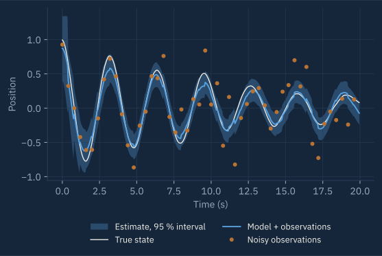
A damped oscillation: true state, noisy observations, and a Kalman-filter estimate with a 95 % band that tracks the true state closely.
Method demonstration. A Kalman filter combines a damped-oscillator model with observations of noise standard deviation 0.25. Position error falls from 0.27 (raw observations) to 0.08 (filtered).

04 / Anomaly Detection

Identify behaviour inconsistent with expected physical or statistical patterns.

The problemA threshold on raw data cannot tell a cloudy day from a fault. Comparing measurements with what physics predicts for the conditions, and flagging only departures larger than the prediction's uncertainty, separates the two.
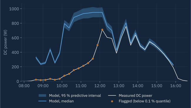
Evidence: CASE / 001

Measured solar array power on 25 December 2012 sits far below the model's predictive band in the morning, with flagged points, and rejoins the band after midday.
From CASE / 001: measured power on a sub-zero morning falls below the model's predictive band and is flagged; after midday it returns inside the band.

05 / Experimental Design

Use quantitative information to guide measurement and experimentation.

The problemMeasurements cost time and money, and not all are equally informative. Expected information about the quantity of interest shows where and when to measure before the experiment is run.
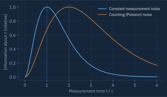
Relative information about a decay time constant against measurement time: it peaks at one time constant for constant noise and at two for counting noise.
Method demonstration. For a decay curve, a single measurement is most informative about the time constant τ at t = 1.0 τ when noise is constant, but at t = 2.0 τ when it is counting noise. The noise model changes the design.

06 / Uncertainty Quantification

Characterise confidence, sensitivity and uncertainty in quantitative results.

The problemEvery input to a calculation is known only approximately. Propagating those uncertainties through the model gives an interval for the result and shows which input dominates it.
Evidence: NOTE / 001

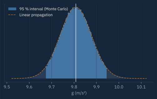
Monte Carlo distribution of g from a pendulum measurement with its central 95 % interval shaded and the linear-propagation curve overlaid.
From NOTE / 001: g = 9.81 ± 0.07 m/s² from a pendulum, with timing contributing 92 % of the variance.

07 / Risk-Informed Decisions

Connect quantitative predictions and uncertainty with decision-making.

The problemA point forecast below a limit can still carry an unacceptable chance of exceeding it. Decisions improve when the whole predictive distribution is weighed against the costs of acting and of not acting.
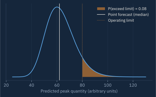
A predictive distribution whose median lies below an operating limit, with the tail beyond the limit shaded; the exceedance probability is 0.08.
Illustration with stated numbers. The median forecast (62) is below the limit (80), yet the probability of exceeding it is 0.08. If protective action costs 5 % of the loss it prevents, acting is the better decision.